GAMS Tutorial #1
← ChE 477: Process Optimization
- Chemical Engineering Optimization Models with GAMS CACHE DESIGN CASE STUDIES SERIES Case Study No.6 1991 Editor: Ignacio E. Grossmann Introduction to GAMS Ignacio E. Grossmann Department of Chemical Engineering Carnegie Mellon University Pittsburgh, PA 15213 GAMS is a modeling system for optimization that provides an interface with a variety of different algorithms. Models are supplied by the user to GAMS in an input file in the form of algebraic equations using a higher level language. GAMS then compiles the model and interfaces automatically with a "solver" (i.e., optimization algorithm). The compiled model as well as the solution found by the solver are then reported back to the user through an output file. The simple diagram below illustrates this process.
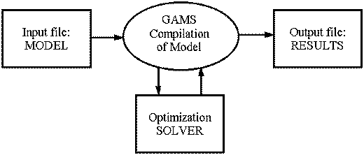 The conventions for naming the extensions of the files are as follows:
Input file: Filename.GMSOutput file: Filename.LSTIn order to compile and execute the input file, the command is simply:GAMS filenameThe GAMS input file is in general organized into the following sections: Specification of indices and data. Listing of names and types of variables and equations (constraints and objective function). Definition of the equations (constraints and objective function). Specification of bounds, initial values and special options. Call to the optimization solver. The format of the input files is not rigid (although the syntax is) as the reader will verify with the GAMS listings provided in this case study. Also, there is a rather large number of keywords so as to provide the flexibility for handling simple and complex models (all in equation form, however, since routines or procedures cannot be handled). In order to provide e brief overview of the syntax for the input file in GAMS we will present two simple example problems. For a detailed description the user should read "GAMS-A User's Guide" by Brooke, Kendrick and Meeraus which is provided with this case study. Example 1 Consider the following nonlinear programming (NLP) problem that is given in Prob1em 8.26 in the book "Engineering Optimization" by Reklaitis, Ravindran and Ragsdell (1983):minimize Z = x12 + x22 + x32s.t. 1-x2-1x3 > 0x1-x3 > 0x1-x22+x2x3-4 = 00 < x1 < 50 < x2 < 30 < x3 < 3 (1)Initial starting point:x1 = 4x2 = 2x3 = 2First we should note that the inequality1-x2-1x3 > 0 (2)can actually be rearranged in linear form as:x2-x3 > 0 (3)Using (3) instead of (2) is a much better choice, not only because we avoid the potential for a division by zero, but also because we obtain a linear constraint which is easier to handle. The GAMS input file TEST.GMS for the rearranged problem in (1) is given in the next page (click on the "TEST.GMS"). First note that the$sign in column 1 is a control directive, the first for specifying the title, the other two for suppressing some details in the output (e.g., map of symbols). In general, you will always include these keywords (see also pp.112-113, GAMS User's Guide). The keywordVARIABLESis used to list our variablesx1, x2andx3. Note thatZ, the objective function value must also be included. The keywordPOSITIVE VARIABLESis used to specify the non-negativity ofx1, x2, x3. The objective function values should not be included here as in general it might take positive or negative values. Finally, note that the semicolon;must be included to specify the end of the lists. Next, the keywordEQUATIONSis for listing the names of the constraints and objective function. The names are arbitrary and here we have selected the namesCON1, CON2, CON3, for the constraints, andOBJfor the objective function. The actual equations are then defined by first listing the name followed by two periods. Note that the following syntax must be used for the equality and inequality signs:=E=for==G=for >=L=for<Also note that the basic arithmetic operators are:+ addition- subtraction∗ multiplication/ division∗∗ exponentIn the objective we could have expressed the equation as:OBJ .. Z = E = X1∗∗2 + X2∗∗2 + X3∗∗2 ;Note the semi-colon;is needed at the end. Also, for illustration purposes, we have used the functionSQRwhich performs the square of the variables. Table 6.1 in p.69 of the User's Guide gives a comp1ete listing of the standard functions that are available in GAMS. Next in the input file we specify the upper bounds and initial values. This is done by adding a subfield to the variables. The format is a period followed by a character, and they are as follows:.LOlower bound.UPupper bound.Llevel value, meaning actual value (initial or final).Mdual prices, Lagrange or Kuhn-Tucker multipliers Note that we do not need to specify lower bounds of zero for x1, x2, x3, because we used the keywordPOSITIVE VARIABLESbefore. Also, it is not a requirement to always specify initial values for the variables. If we do not, then GAMS will set them to the lower bounds. For nonlinear problems, however, it is often advisable to supply an initial guess (e.g., seeX1.L= 4;). The keywordMODELis used to name our model and to specify which equations should be used. In this case we name our model as TEST and specify that all equations be used. Next, theOPTIONstatements are used to suppress output for debugging the compilation of the equations. Pages 102-106 in the User's Guide gives a detailed explanation of this keyword. Suffice it to say that in most cases you want to use both theOPTION LIMROW = 0andOPTION LIMCOL = 0to avoid long output files. Finally, we invoke the optimization algorithm with theSOLVEstatement. Here the format is as follows:SOLVE(model name)USING(solver type)MINIMIZING(objective variable) orSOLVE(model name)USING(solver type)MAXIMIZING(objective variable) TEST.GMS$TITLE Test Problem$OFFSYMXREF$OFFSYMLIST∗ Example from Problem 8.26 in "Engineering Optimization"∗ by Reklaitis, Ravindran and Ragsdell (1983)∗VARIABLES X1, X2, X3, Z ;POSITIVE VARIABLES X1, X2, X3 ;EQUATIONS CON1, CON2, CON3, OBJ ;CON1.. X2 - X3 =G= 0 ;CON2.. X1 - X3 =G= 0 ;CON3.. X1 - X2∗∗2 + X1∗X2 - 4 =E= 0 ;OBJ.. Z =E= SQR(X1) + SQR(X2) + SQR(X3) ;∗ Upper boundsX1.UP = 5 ;X2.UP = 3 ;X3.UP = 3 ;∗ Initial pointX1.L = 4 ;X2.L = 2 ;X3.L = 2 ;MODEL TEST / ALL / ;OPTION LIMROW = 0;OPTION LIMCOL = 0;SOLVE TEST USING NLP MINIMIZING Z;Back The main solver types available in GAMS are as follows:LPlinear programmingNLPnonlinear programmingMIPmixed-integer linear programmingRMIPrelaxed MILP where the integer variables are treated as continuousMINLPmixed-integer nonlinear programming in which the integer variables are 0-1 and linear; the continuous variables can be nonlinearRMINLPmixed-integer nonlinear programming where the integer variables are treated as continuous The optimization software provided in this case study is as follows for each solver type (default options):LPBDMLPMIP, RMIPZOOMNLPMINOS5.3MINLPDICOPT++ BDMLP uses the simplex algorithm for linear programming; so does ZOOM with the branch and bound method for MILP. MINOS5.3 makes use of the reduced gradient method with augmented Lagrangian for NLP, which reduces to the simplex algorithm when the objective function and constraints are linear. Finally, DICOPT++ is based on the augmented penalty version of the outer-approximation method for MINLP. A description of the simplex algorithm, the branch and bound method and the reduced gradient method can be found in the bibliography supplied in the appendix. The appendix also contains a description of the method behind DICOPT++. GAMS bas a default for selecting each optimization algorithm. It is the first in the above list. If we wish to select another algorithm, say ZOOM instead of BDMLP when solving an LP, this is specified with the statement:OPTION LP = ZOOM ;If we now run GAMS with our input file TEST.GMS (type GAMS TEST) we obtain the output file TEST.LST which is shown in the next two pages (click on the "TEST.LST"). Note that the first pan of the output is identical to the input file (lines 4 to 36). Next, statistics on the problem size are reported (e.g., 4 variables: x1, x2, x3, Z; 4 equations: 3 constraints and objective). The derivative pool refers to the fact that analytical gradients for the nonlinear model have been generated by GAMS. The solve summary indicates that the optimum bas been found (local because it is an NLP) with an objective function value Z = 7.2177. Resource usage indicates the solver MINOS took 1.648 secs. A detailed explanation of the other output in this sections can be found in pp.117-119 of the User's Guide. Finally, information on the equations and variables are listed. The column labeledLEVELgives the actual values. So for instanceX1 = 2.526, X2=0.916, X3= 0, Z = 7.218. The columnsLOWERandUPPERgive the lower and upper bounds, while the columnMARGINALgives the dual variables or multipliers. So for insistence, the third constraint (CON3) has s multiplier of 2.637 as the equation is an active constraint. The first two constraints have zero multipliers since they are not active at the lower or upper bounds. More details on the output can be found in pp.120-121 of the User's Guide. TEST.LSTGAMS 2.25 PC AT/XT 09/16/9723:48:05 PAGE 1Test Problem45 ∗ Example from Problem 8.26 in "Engineering Optimization"6 ∗ by Reklaitis, Ravindran and Ragsdell (1983)7 ∗89 VARIABLES X1, X2, X3, Z ;10 POSITIVE VARIABLES X1, X2, X3 ;1112 EQUATIONS CON1, CON2, CON3, OBJ ;1314 CON1.. X2 - X3 =G= 0 ;15 CON2.. X1 - X3 =G= 0 ;16 CON3.. X1 - X2∗∗2 + X1∗X2 - 4 =E= 0 ;17 OBJ.. Z =E= SQR(X1) + SQR(X2) + SQR(X3) ;1819 ∗ Upper bounds20 X1.UP = 5 ;21 X2.UP = 3 ;22 X3.UP = 3 ;2324 ∗ Initial point25 X1.L = 4 ;26 X2.L = 2 ;27 X3.L = 2 ;2829 MODEL TEST / ALL / ;3031 OPTION LIMROW = 0;32 OPTION LIMCOL = 0;3334 SOLVE TEST USING NLP MINIMIZING Z;COMPILATION TIME = 0.060 SECONDS VERID TP5-00-038GAMS 2.25 PC AT/XT 09/16/9723:48:05 PAGE 2Test ProblemModel Statistics SOLVE TEST USING NLP FROM LINE 34MODEL STATISTICSBLOCKS OF EQUATIONS 4 SINGLE EQUATIONS 4BLOCKS OF VARIABLES 4 SINGLE VARIABLES 4NON ZERO ELEMENTS 10 NON LINEAR N-Z 5DERIVATIVE POOL 6 CONSTANT POOL 2CODE LENGTH 57GENERATION TIME = 0.000 SECONDSEXECUTION TIME = 0.110 SECONDS VERID TP5-00-038GAMS 2.25 PC AT/XT 09/16/9723:48:05 PAGE 3Test ProblemSolution Report SOLVE TEST USING NLP FROM LINE 34S O L V E S U M M A R YMODEL TEST OBJECTIVE ZTYPE NLP DIRECTION MINIMIZESOLVER MINOS5 FROM LINE 34∗∗∗∗ SOLVER STATUS 1 NORMAL COMPLETION∗∗∗∗ MODEL STATUS 2 LOCALLY OPTIMAL∗∗∗∗ OBJECTIVE VALUE 7.2177RESOURCE USAGE, LIMIT 0.336 1000.000ITERATION COUNT, LIMIT 15 1000EVALUATION ERRORS 0 0M I N O S 5.3 (Nov 1990) Ver: 225-DOS-02= = = = =B. A. Murtagh, University of New South WalesandP. E. Gill, W. Murray, M. A. Saunders and M. H. WrightSystems Optimization Laboratory, Stanford University.D E M O N S T R A T I O N M O D EYou do not have a full license for this program.The following size retrictions apply:Total nonzero elements: 1000Nonlinear nonzero elements: 300Estimate work space needed -- 39 KbWork space allocated -- 160 KbEXIT -- OPTIMAL SOLUTION FOUNDMAJOR ITNS, LIMIT 7 200FUNOBJ, FUNCON CALLS 34 34SUPERBASICS 1INTERPRETER USAGE .00NORM RG / NORM PI 9.678E-10LOWER LEVEL UPPER MARGINAL---- EQU CON1 . 0.916 +INF .---- EQU CON2 . 2.526 +INF .---- EQU CON3 4.000 4.000 4.000 2.637---- EQU OBJ . . . 1.000LOWER LEVEL UPPER MARGINAL---- VAR X1 . 2.526 5.000 .---- VAR X2 . 0.916 3.000 EPS---- VAR X3 . . 3.000 EPS---- VAR Z -INF 7.218 +INF .∗∗∗∗ REPORT SUMMARY : 0 NONOPT0 INFEASIBLE0 UNBOUNDED0 ERRORSGAMS 2.25 PC AT/XT 09/16/9723:48:05 PAGE 4Test ProblemSolution Report SOLVE TEST USING NLP FROM LINE 34EXECUTION TIME = 0.050 SECONDS VERID TP5-00-038USER: CACHE DESIGN CASE STUDIES SERIES G911007-1447AX-TP5GAMS DEMONSTRATION VERSION∗∗∗∗ FILE SUMMARYINPUT C:\GAMS\TEST.GMSOUTPUT C:\GAMS\TEST.LSTBack Example 2 Consider the problem of assigning process streams to heat exchangers as described in pp.409-410 of the book "Optimization of Chemical Process" by Edgar and Himmelblau. The optimization problem is given by:minimize Z =SiSj Cijxijs.t.Si xij=1 j=l,...,nSj xij=1 i=l,...,n (4)xij=0,1 i=l,...,n & j=l,...,nwhich corresponds to the well known assignment problem. Here i represents. the index for the n streams and j the index for the n exchangers. The binary variable xij=1 if stream i is assigned to exchanger j, and xij=0 if it is not. The two equations simply state that every exchanger j must be assigned to one stream. and every stream i must be assigned to one exchanger. The cost Cij of assigning stream i to exchanger j is as follows:ExchangersStreams 1 2 3 4A 94 1 54 68B 74 10 88 82C 73 88 8 76D 11 74 81 21We can formulate the above problem in GAMS in the form of the model in (4) using index sets (click on the HEAT.GMS to see the input file). As shown in the output file HEAT.LST in the next page (click on the "HEAT.LST" to see the output file), the structure of this file is similar to the one of Example 1, except for the use of indices. Note that the data are given in terms ofSETSand theTABLE. (see pp.43-47 and pp.53-57 in the User's Guide). The elements of a set can be names (A, B, C, D) or numbers. In the latter case we can use the∗sign to denote the range (1∗4, means 1, 2, 3, 4). For theTABLEthere is no need to place the numbers in precise positions; they only have to be consistent, Data can also be entered using the keywordsSCALARandPARAMETERS(see p.53 and pp.51-53 of the User's Guide). Note that we can specify xij as a variable with indices,X(I,J), and similarly the two equations:ASSI(J)means forj = 1, 2, 3, 4;ASSJ(I)means fori = A, B, C, D. Also, in this case since xij is restricted to 0-1 values, we use the keywordBINARY VARIABLES. The summation is expressed in the form ofSUM(index of summation, terms in sum) (see pp.17.18 of User's Guide). Last, for the input, we have used theOPTION SOLPRINT=OFFstatement, so as to only print the values of the variables xij and the objectiveZ. This is done with theDISPLAYkeyword where we list the level value of the xij (X.L- no indices are needed) and of Z (Z.L). More information onDISPLAYcan be found in pages 143-148 of the user's guide. Finally, note that in theSOLVEstatement we specify the solverMIPdue to the fact that the xij are binary variables. The solve summary indicates that the optimum objective function is Z=97. We also note that the solution was obtained from the relaxed LP. This is nor surprising since it is well known that the assignment problem has a "unimodular" matrix and therefore the solutions for the xij are guaranteed to be 0-1 if we solve the problem as an LP (you may try this as a simple experiment). Finally, due to the use of theDISPLAYstatement the requested variables are printed. Note that stream A is assigned to exchanger 4, B to 2, C to 3, and D to 1, with a minimum cost of 97. HEAT.GMS$TITLE Test Problem$OFFSYMXREF$OFFSYMLIST∗∗ Assignment problem for heat exchangers from pp.409-410 in∗ Optimization of Chemical Processes" by Edgar and Himmelblau∗SETSI streams / A, B, C, D /J exchangers / 1∗4 / ;TABLE C(I,J) Cost of assigning stream i to exchanger j1 2 3 4A 94 1 54 68B 74 10 88 82C 73 88 8 76D 11 74 81 21 ;VARIABLES X(I,J), Z;BINARY VARIABLES X(I,J);EQUATIONS ASSI(J), ASSJ(I), OBJ;ASSI(J).. SUM( I, X(I,J) ) =E= 1;ASSJ(I).. SUM( J, X(I,J) ) =E= 1;OBJ.. Z =E= SUM ( (I,J), C(I,J)∗X(I,J) ) ;MODEL HEAT / ALL /;OPTION LIMROW = 0;OPTION LIMCOL = 0;OPTION SOLPRINT = OFF;SOLVE HEAT USING MIP MINIMIZING Z;DISPLAY X.L, Z.L ;Back HEAT.LSTGAMS 2.25 PC AT/XT 09/16/9723:53:18 PAGE 1Test Problem45 ∗6 ∗ Assignment problem for heat exchangers from pp.409-410in7 ∗ Optimization of Chemical Processes" by Edgar andHimmelblau8 ∗910 SETS11 I streams / A, B, C, D /12 J exchangers / 1∗4 / ;1314 TABLE C(I,J) Cost of assigning stream i to exchanger j1516 1 2 3 417 A 94 1 54 6818 B 74 10 88 8219 C 73 88 8 7620 D 11 74 81 21 ;212223 VARIABLES X(I,J), Z;24 BINARY VARIABLES X(I,J);2526 EQUATIONS ASSI(J), ASSJ(I), OBJ;2728 ASSI(J).. SUM( I, X(I,J) ) =E= 1;29 ASSJ(I).. SUM( J, X(I,J) ) =E= 1;30 OBJ.. Z =E= SUM ( (I,J), C(I,J)∗X(I,J) ) ;3132 MODEL HEAT / ALL /;3334 OPTION LIMROW = 0;35 OPTION LIMCOL = 0;36 OPTION SOLPRINT = OFF;3738 SOLVE HEAT USING MIP MINIMIZING Z;3940 DISPLAY X.L, Z.L ;COMPILATION TIME = 0.060 SECONDS VERID TP5-00-038GAMS 2.25 PC AT/XT 09/16/9723:53:18 PAGE 2Test ProblemModel Statistics SOLVE HEAT USING MIP FROM LINE 38MODEL STATISTICSBLOCKS OF EQUATIONS 3 SINGLE EQUATIONS 9BLOCKS OF VARIABLES 2 SINGLE VARIABLES 17NON ZERO ELEMENTS 49 DISCRETE VARIABLES 16GENERATION TIME = 0.050 SECONDSEXECUTION TIME = 0.160 SECONDS VERID TP5-00-038GAMS 2.25 PC AT/XT 09/16/9723:53:18 PAGE 3Test ProblemSolution Report SOLVE HEAT USING MIP FROM LINE 38S O L V E S U M M A R YMODEL HEAT OBJECTIVE ZTYPE MIP DIRECTION MINIMIZESOLVER ZOOM FROM LINE 38∗∗∗∗ SOLVER STATUS 1 NORMAL COMPLETION∗∗∗∗ MODEL STATUS 1 OPTIMAL∗∗∗∗ OBJECTIVE VALUE 97.0000RESOURCE USAGE, LIMIT 0.047 1000.000ITERATION COUNT, LIMIT 16 1000Z O O M / X M P --- PC Version 2.2 Nov 1990Dr Roy E. Marsten and Dr Jaya Singhal,XMP Optimization Software Inc.Tucson, ArizonaD E M O N S T R A T I O N M O D EYou do not have a full license for this program.The following size retrictions apply:Total nonzero elements: 1000Total discrete variables: 20Estimate work space needed -- 16 KbWork space allocated -- 273 KbIterations TimeInitial LP 16 .00Heuristic 0 .00Branch and bound 0 .00Final LP 0 .00∗∗∗∗ REPORT SUMMARY : 0 NONOPT0 INFEASIBLE0 UNBOUNDEDGAMS 2.25 PC AT/XT 09/16/9723:53:18 PAGE 4Test ProblemE x e c u t i o n---- 40 VARIABLE X.L1 2 3 4A 1.000B 1.000C 1.000D 1.000---- 40 VARIABLE Z.L = 97.000EXECUTION TIME = 0.060 SECONDS VERID TP5-00-038USER: CACHE DESIGN CASE STUDIES SERIES G911007-1447AX-TP5GAMS DEMONSTRATION VERSION∗∗∗∗ FILE SUMMARYINPUT C:\GAMS\HEAT.GMSOUTPUT C:\GAMS\HEAT.LSTBack Useful Hints and Information Before you install GAMS and the input files you should read the Appendix "Instructions for Installing GAMS". The version included in this case study will run on an IBM-PC or compatible under the DOS operating system (2.11 or higher). The minimum required free memory is 500K. Therefore, a PC with 1 Megabyte RAM is recommended. Also, a hard disk is required. For several problems a 386 machine or higher is recommended. In terms of size, this version is restricted to problems with up to 1000 nonzero coefficients (maximum of 300 nonlinear) and 20 discrete variables. If you have never used GAMS before, you may want to run the first problem: REFINERY.GMS (type GAMS REFINERY). The results are in the output file REFINERY.LST. You can edit this file for instance with the editor epsilon. Before you run any of the other problems, first read the Appendix "GAMS Input Files" as some of them require more than 10 minutes on a 286 machine. When editing the output file the quickest is to search with your editor for:S O L. This will position yourself in the sectionS O L V E S U M M A R Y. Resource usage refers to the CPU time required by the solver. The best way to learn the syntax In GAMS is to type in the files TEST.GMS and HEAT.GMS of this introduction section. Can you reproduce the some results? GAMS is somewhat fuzzy with the syntax. When creating your own file it is not unusual that GAMS will complain the first time. Watch for the=E=,=L=,=G=, signs in your equations and inequalities. Also, do not omit semi-colons at the end of them. Also, watch for the correct number of parenthesis. If you intend to use the MINLP solver DICOPT++, read first that Appendix, and type in by yourself the file HW3JV.GMS. Also, only use 0-1 variables that are linear (i.e. do not multiply a binary by a continuous variable!). If you intend to solve problems with Benders decomposition or solve differential/algebraic problems, read the corresponding Appendices provided for this case study. Final Remarks The two examples given in this introduction have only covered the basic elements for the GAMS language. Two other useful operators that the reader will find in several of the problems of this case study are: Dollar operator ($) which is used to restrict the elements in a set (see pp.72-76 of the User's Guide).LOOPkeyword which can be used as a DO statement in FORTRAN to either perform repetitive calculations or multipleSOLVEstatements (sec pp.138-140 of User's Guide). It is also useful to point out that GAMS is available on a number of different computer platforms which range from PC's and workstations to mainframes. Larger versions of GAMS are available. Information on GAMS can be obtained from Scientific Press, 651 Gateway Boulevard, Suite 1100, South San Francisco, CA 94080-7014. Tel: (415) 583-6371; Fax: (415) 583-6371.