MATLAB: contourconstraint
← ChE 477: Process Optimization
close all
clear all
clc

% PLOT CONTOURS & INEQUALITY & EQUALITY CONSTRAINTS
% Modified by Ugur Akman 2004

%	Chapter 2: Optimization with Matlab
%  Dr. P.Venkataraman
%  Example 1 (Sec 2.1- 2.2)
%
%	graphical solution using matlab (two design variables)
%	the following script should allow the graphical solution
%	to example [ problem 3-90 from text]
%
%	Minimize	f(x1,x2) = (x1-3)**2 + (x2-2)**2
%
%				h1(x1,x2) = 2x1 + x2 = 8
%				h2(x1,x2) = (x1-1)^2 + (x2-4)^2 = 4
%				g1(x1,x2) : x1 + x2 <= 7
%				g1(x1,x2) : x1 - 0.25x2^2 <= 0.0
%
%			0 <= x1 <= 10 ; 0 <= x2 <= 10
%
%
%	WARNING : The hash marks for the inequality constraints must
%			be determined and drawn outside of the plot
%			generated by matlab
%
%----------------------------------------------------------------

x1=0:0.1:10;	% the semi-colon at the end prevents the echo
x2=0:0.1:10;	% these are also the side constraints
% x1 and x2 are vectors filled with numbers starting
% at 0 and ending at 10.0 with values at intervals of 0.1

[X1 X2] = meshgrid(x1,x2);
% generates matrices X1 and X2 corresponding vectors x1 and x2

f1 = (X1 - 3).*(X1 - 3) +(X2 - 2).*(X2 - 2);
% the objecive function is evaluated over the entire mesh

ineq1 = X1 + X2;
% the inequality g1 is evaluated over the mesh
ineq2 = X1 - 0.25*X2.^2;
% the inequality g2 is evaluated over the mesh

eq1 = 2.0*X1 + X2;
% the equality 1 is evaluated over the mesh
eq2 = (X1 - 1).*(X1 - 1) + (X2 - 4).*(X2 - 4);
% the equality 2 is evaluated over the mesh

[C1,h1] = contour(x1,x2,ineq1,[7,7],'r-','LineWidth',2);
clabel(C1,h1);
hold on	% allows multiple plots
% ineq1 is plotted [at the contour value of 7] RED
% NOTE: You may define ineq1 (g1) as:
%          ineq1 = X1 + X2 - 7
%       and plot the zero-valued contour as:
%          [C1,h1] = contour(x1,x2,ineq1,[0,0],'r-');
%          clabel(C1,h1);

[C2,h2] = contour(x1,x2,ineq2,[0,0],'m-','LineWidth',2);
clabel(C2,h2);
% ineq2 is plotted [at the contour value of 0] PURPLE

[C3,h3] = contour(x1,x2,eq1,[8,8],'b-','LineWidth',2);
clabel(C3,h3);
% eq1 is plotted [at the contour value of 8] BLUE
% NOTE: See the above note

[C4,h4] = contour(x1,x2,eq2,[4,4],'k-','LineWidth',2);
clabel(C4,h4);
% eq2 is plotted [at the contour value of 4] BLACK
% NOTE: See the above note

[C,h] = contour(x1,x2,f1,'g-','LineWidth',2);
clabel(C,h);
% obj fct contours are plotted GREEN

xlabel(' x1 values','FontName','times','FontSize',12,'FontWeight','bold');
% label for x-axes
ylabel(' x2 values','FontName','times','FontSize',12,'FontWeight','bold');
% label for y-axes

grid
hold off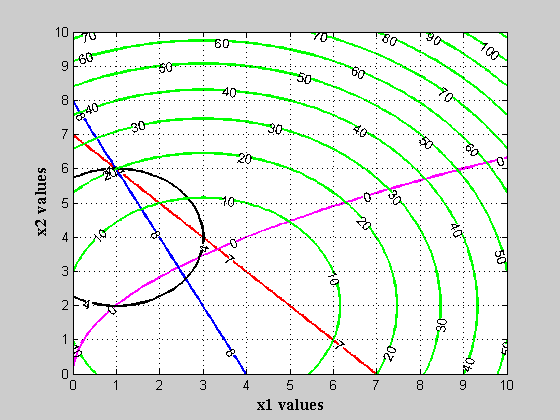
Published with MATLAB® 7.0