MATLAB: ex1
← ChE 555: Applied Mathematics & Modeling for Chemical Engineers
echo off;
clc;
clear all;
close all;

% Initial value of indepemdent variable (t0)
% Final value of independent variable (tf)
% Initial value of dependent variable (y0)
% Integration error tolerance (tol)
t0 = 0;
tf = 3;
y0 = 0;

% Define the integration options
% see ode23 help
options = odeset('RelTol',1e-4,'AbsTol',[1e-5],'Stats','on');

% Integrate by ODE23 the derivative functions
% defined in the file EX1F.M and assign the
% solution vector to maxrix [t,y]
[t,y] = ode23 ('ex1f',[t0 tf],y0,options);

% NOTE:
% Integrate by ODE23 the derivative functions
% defined within this file as "inline"
% (wihtout writing another .m file)
%        dydt=inline('-2*t*y+4*t');
%        [t,y] = ode23 (dydt,[t0 tf],y0,options);

% Evaluate the analytical solution and assign
% the solution vector to vector [yanalytic]
constant = (y0-2)/exp(-t0^2);
yanalytic = 2+constant*exp(-diag(t)^2);

% Plot the numerical solution vector [t,y] with red ('r') line ('-')
figure
plot(t,y,'r-');
title('ChE585 EXAMPLE-1'); grid;
xlabel('x-axis'); ylabel('y-axis');
text(2.2,0.3,'red: numerical');

% Hold the current graph to plot the analytical solution on the same graph
hold on;

% Plot the analytical solution vector
% [t,diagonal(yanalytic)] with blue ('b') circles ('-')
plot(t,diag(yanalytic),'bo');
text(2.2,0.1,'blue: analytical');
30 successful steps
6 failed attempts
109 function evaluations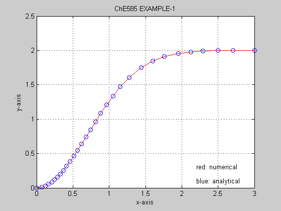
Published with MATLAB® 7.0