MATLAB Example 3
← ChE 555: Applied Mathematics & Modeling for Chemical Engineers
- ChE 585 MATLAB Examples EXAMPLE - 3 (A Boundary Value Problem - BVP) In this example we solve the following 3rd order ODE: ODE:
 B.C.s:
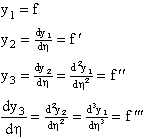
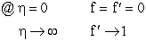 Analytical solution: there is no analytical solution to this nonlinear problem. Since the ODE solvers we have are IVP (Initial Value Problem) solvers for first order ODEs, in order to solve this third order BVP (Boundary Value Problem) we have to convert it into three first order ODEs. Let:
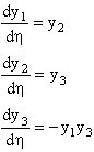
 Then, the original 3rd order ODE can be written as a set of 1st order ODEs:
 Now, the initial conditions on y1 & y2 are known as
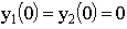 . On the other hand, the initial condition on y3 is not known (i.e., the original problem does not state
 explicitly). However, the boundary condition on y2 (i.e.,
 ) can be used to determine the proper initial condition on y3 (e.g., by trial and error). Practically
 for
 . So, by trial and error, the proper initial condition for y3 is
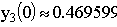 . Program Name: EX3.M clear; % Initial value of indepemdent variable (x0) % Final value of independent variable (xf) % Initial value of dependent variable (y0) % Integration error tolerance (tol) % ------------------------------------------ x0 = 0; xf = 5; y0 = [0 0 0.469599]; tol = 1.e-3; trace = 0; % % Integrate by ODE45 the derivative functions % defined in file EX3-F.M and assign the % solution vector to maxrix [x,y] % -------------------------------------------- [x,y] = ode45 ('ex3-f',x0,xf,y0,tol,trace); % % Plot the numerical solution vector [x,y] % ----------------------------------------- hold; plot(x,y(:,1),'r-'); plot(x,y(:,2),'y-'); plot(x,y(:,3),'g-'); title('ChE585 EXAMPLE-3'); grid; xlabel('x-axis'); ylabel('y-axis'); text(0.5,3.75,'red: y(1)=f, numerical'); text(0.5,3.25,'yellow: y(2)=dfdeta, numerical'); text(0.5,2.75,'green: y(3)=d2fdeta2, numerical'); Function Name: EX3-F.M function dydx = ode (x,y) % Define the derivative vector dydx=[dy1dx dy2dx dy3dx] dydx = [y(2) y(3) -y(1)∗y(3)];